The mathematical viral infection model used in the accompanying blog
Last updated 28 October 2021
It is not possible to use subscripts on this page. The pdf or docx downloads do contain the necessary subscripts.
(c) michaeljcole@hotmail.com. Please copy, quote or publish this material for any non-commercial purpose, with attribution.
It is not possible to use subscripts on this page. The pdf or docx downloads do contain the necessary subscripts.
(c) michaeljcole@hotmail.com. Please copy, quote or publish this material for any non-commercial purpose, with attribution.
Download a docx or pdf of this page here: Temporarily unavailable during updating.
The Epidemic Model
A simple Model
A simple formula for new daily cases of an infection, if the maximum effective incubation period, i, is 6 days, is:
N t+i = (Nt+5 + Nt+4 + Nt+3 + Nt+2 + Nt+1 + Nt ) * Rs /i * (P – Cumulative Cases t+5)/P
where N t+6 (N at day t+i) is obtained by dividing the number of infecting cases (the sum of N between day t+0 and day t+5) by the maximum effective incubation period (6 days) and then multiplying by Rs (the effective R amongst the still susceptible) and then multiplying by the proportion of the population still susceptible to the infection (P, the population, minus the cumulative cases to date, as a proportion of P). N t+6, in this case, is N (t+the maximum effective incubation period).
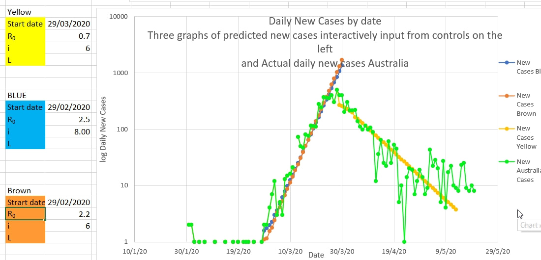
Rs and the maximum effective number of infecting days can be obtained by plotting (on log scale) the number of new cases predicted by this simple model (seeded with actual case numbers) and using various values of Rs and i, to obtain the 'best fit' to a plot of the actual daily cases. On this interactive chart below, Rs (incorrectly labelled R₀) and i are easily estimated by finding the best fit. That is, finding the best fit of a projection using guesses of Rs and i to the actual cases.
Prior to restrictions (non pharmacologic interventions) being introduced, Rs closely approximates R₀. But after restriction are introduced Rs (the effective R amongst the susceptible) decreases. Early in the wave Rs, and therefore R₀, was estimated at between 2.2 and 2.5, and the maximum effective incubation period as between 6 and 8 days. After the peak of the wave, NPI (restrictions) had reduced Rs to 0.7
A simple formula for new daily cases of an infection, if the maximum effective incubation period, i, is 6 days, is:
N t+i = (Nt+5 + Nt+4 + Nt+3 + Nt+2 + Nt+1 + Nt ) * Rs /i * (P – Cumulative Cases t+5)/P
where N t+6 (N at day t+i) is obtained by dividing the number of infecting cases (the sum of N between day t+0 and day t+5) by the maximum effective incubation period (6 days) and then multiplying by Rs (the effective R amongst the still susceptible) and then multiplying by the proportion of the population still susceptible to the infection (P, the population, minus the cumulative cases to date, as a proportion of P). N t+6, in this case, is N (t+the maximum effective incubation period).
Rs and the maximum effective number of infecting days can be obtained by plotting (on log scale) the number of new cases predicted by this simple model (seeded with actual case numbers) and using various values of Rs and i, to obtain the 'best fit' to a plot of the actual daily cases. On this interactive chart below, Rs (incorrectly labelled R₀) and i are easily estimated by finding the best fit. That is, finding the best fit of a projection using guesses of Rs and i to the actual cases.
Prior to restrictions (non pharmacologic interventions) being introduced, Rs closely approximates R₀. But after restriction are introduced Rs (the effective R amongst the susceptible) decreases. Early in the wave Rs, and therefore R₀, was estimated at between 2.2 and 2.5, and the maximum effective incubation period as between 6 and 8 days. After the peak of the wave, NPI (restrictions) had reduced Rs to 0.7
Improved Model
A simple formula for estimating new daily cases of COVID-19 can be improved because it has now been shown that the incubation period is 1 to 14 days, and the probability of the incubation taking a particular number of days is known.
A simple formula for estimating new daily cases of COVID-19 can be improved because it has now been shown that the incubation period is 1 to 14 days, and the probability of the incubation taking a particular number of days is known.
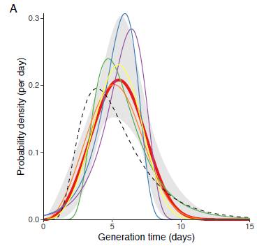
Luca Ferretti, Alice Ledda, Chris Wymant et al, ‘The timing of COVID-19 transmission’, September 16, 2020, medRxiv online. At https://doi.org/10.1101/2020.09.04.20188516
The generation time of Covid-19 (from infected to infected). The incubation period (from infection to symptoms (if any) is shown as a dotted line).
|
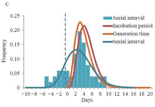
Meng Zhang et al, 'Transmission Dynamics of an Outbreak of the COVID-19 Delta Variant B.1.617.2 — Guangdong Province, China, May–June 2021', July 2021. At https://www.ncbi.nlm.nih.gov/pmc/articles/PMC8392962/pdf/ccdcw-3-27-584.pdf |
The probability of the incubation being 1 day long is very low, so the probability of having been infected by cases reported the day before are very low. The probability of the incubation being 2 days long is 8.8 percent, so the probability of being infected by the cases reported 2 days before the symptoms is 0.088 or 8.8 percent. And etc for the other days. The probability of having been infected 1 day before or 11 to 15 days before are low, so are not used, although they could be, in this application of the Model. Only the probabilities of infection for days 2 to 10 (numbered t, t+1 etc to t+8) are used in this Model. The probabilities for these 9 days were adjusted (normalised to add up to 1 (100%) since you can’t be infected more or less than 100%. These adjusted probabilities are used as coefficients, to multiply by the number of reported cases on that day.
The normalised probability, a, of being infected 1, 2 , 3 etc to 10 days before symptoms ('at' to 'at+8') has been shown to be 0, 0.092, 0.19, 0.20, 0.18, 0.13, 0.092, 0.058, 0.037.
So the final equation for Covid-19 (Equation A) is:
N t+10 = (0.092 Nt+8 + 0.190 Nt+7 + 0.200 Nt+6 + 0.180 Nt+5 + 0.130 Nt+4 + 0.092 Nt+3 + 0.058 Nt+2 + 0.037 Nt+1) * Rs *
(P – C t+9)/P
Where C t+9 is the cumulative total cases (all cases) up to day t+9, and
Nt+i is Nt+10 for Covid-19 because, although the maximum incubation period is 15 days, the probability of 1 or 11 to 15 day incubation periods is very low, so the probability of the incubation periods of 2 to 9 days (t+1 to t+8) are used, and normalized to sum to 1.
or,
N t+10 = ADD(ax*Nx for x=t to x=t+8) * Rs * (P – C t+9)/P (Equation A)
Or more formally,
x = t+8
N t+10 = Rs * (P – C t+9)/P * Σ (ax Nx) rearranged (Equation A)
x = t
Where at to at+8 are 0.026, 0.037, 0.058, 0.092, 0.130, 0.180, 0.200, 0.190, and 0.092 respectively.
Since the probabilities (coefficients) are adjusted (normalised) to add up to 1 (100%), it is no longer necessary to divide Rs by i.
Using the frequency distribution of incubation periods from Zhang etc al above, the coefficients for frequencies (probabilities of occurrence) over 0.035 could be used and normalised, in which the new cases on day t+13, (Nt+13), could be calculated from the probabilities of the incubation periods on day 11 to 4. Viz 0.040, 0.138, 0.216, 0.219, 0.170, 0.109, 0.070 and 0.037.
N t+13 = (0.040 Nt+11 + 0.138 Nt+10 + 0.216 Nt+9 + 0.219 Nt+8 + 0.170 Nt+7 + 0.109 Nt+6 + 0.070 Nt+5 + 0.037 Nt+4) * Rs * (P – C t+9)/P
Estimating Rs
If public health measures (restrictions, public health measures) are in place to limit the spread of Covid then the number of cases infected by one case (Rs) will decrease.
An estimated Rs can be obtained by rearranging Equation A,
N t+10 = (at+8*Nt+8 + at+7*Nt+7 + at+6*Nt+6 + at+5*Nt+5 + at+4*Nt+4 + at+3*Nt+3 + at+2*Nt+2 + at+1*Nt+1 + at*Nt ) * Rs * (P – C t+9)/P (Equation A)
Rs = N t+10 / (0.092 Nt+8 + 0.190 Nt+7 + 0.200 Nt+6 + 0.180 Nt+5 + 0.130 Nt+4 + 0.092 Nt+3 + at+2 Nt+2 + 0.058 Nt+1 + 0.037Nt) * P/(P – C t+9)
or more formally,
x = t+8
Rs = N t+10 * (P / (P – C t+9)) / ( Σ (ax Nx) ) Equation B
x = t
where Nt+10 means N sub-scripted at time t+10, P is the population, Ct+9 is the cumulative total cases on sub-scripted time t+9, ax is a at sub-script time x and Nx is N at sub-script time x.
The reported New Cases each day show ‘noise’ and are probably caused by delays in tracing and reporting cases followed by sudden catch up.
The normalised probability, a, of being infected 1, 2 , 3 etc to 10 days before symptoms ('at' to 'at+8') has been shown to be 0, 0.092, 0.19, 0.20, 0.18, 0.13, 0.092, 0.058, 0.037.
So the final equation for Covid-19 (Equation A) is:
N t+10 = (0.092 Nt+8 + 0.190 Nt+7 + 0.200 Nt+6 + 0.180 Nt+5 + 0.130 Nt+4 + 0.092 Nt+3 + 0.058 Nt+2 + 0.037 Nt+1) * Rs *
(P – C t+9)/P
Where C t+9 is the cumulative total cases (all cases) up to day t+9, and
Nt+i is Nt+10 for Covid-19 because, although the maximum incubation period is 15 days, the probability of 1 or 11 to 15 day incubation periods is very low, so the probability of the incubation periods of 2 to 9 days (t+1 to t+8) are used, and normalized to sum to 1.
or,
N t+10 = ADD(ax*Nx for x=t to x=t+8) * Rs * (P – C t+9)/P (Equation A)
Or more formally,
x = t+8
N t+10 = Rs * (P – C t+9)/P * Σ (ax Nx) rearranged (Equation A)
x = t
Where at to at+8 are 0.026, 0.037, 0.058, 0.092, 0.130, 0.180, 0.200, 0.190, and 0.092 respectively.
Since the probabilities (coefficients) are adjusted (normalised) to add up to 1 (100%), it is no longer necessary to divide Rs by i.
Using the frequency distribution of incubation periods from Zhang etc al above, the coefficients for frequencies (probabilities of occurrence) over 0.035 could be used and normalised, in which the new cases on day t+13, (Nt+13), could be calculated from the probabilities of the incubation periods on day 11 to 4. Viz 0.040, 0.138, 0.216, 0.219, 0.170, 0.109, 0.070 and 0.037.
N t+13 = (0.040 Nt+11 + 0.138 Nt+10 + 0.216 Nt+9 + 0.219 Nt+8 + 0.170 Nt+7 + 0.109 Nt+6 + 0.070 Nt+5 + 0.037 Nt+4) * Rs * (P – C t+9)/P
Estimating Rs
If public health measures (restrictions, public health measures) are in place to limit the spread of Covid then the number of cases infected by one case (Rs) will decrease.
An estimated Rs can be obtained by rearranging Equation A,
N t+10 = (at+8*Nt+8 + at+7*Nt+7 + at+6*Nt+6 + at+5*Nt+5 + at+4*Nt+4 + at+3*Nt+3 + at+2*Nt+2 + at+1*Nt+1 + at*Nt ) * Rs * (P – C t+9)/P (Equation A)
Rs = N t+10 / (0.092 Nt+8 + 0.190 Nt+7 + 0.200 Nt+6 + 0.180 Nt+5 + 0.130 Nt+4 + 0.092 Nt+3 + at+2 Nt+2 + 0.058 Nt+1 + 0.037Nt) * P/(P – C t+9)
or more formally,
x = t+8
Rs = N t+10 * (P / (P – C t+9)) / ( Σ (ax Nx) ) Equation B
x = t
where Nt+10 means N sub-scripted at time t+10, P is the population, Ct+9 is the cumulative total cases on sub-scripted time t+9, ax is a at sub-script time x and Nx is N at sub-script time x.
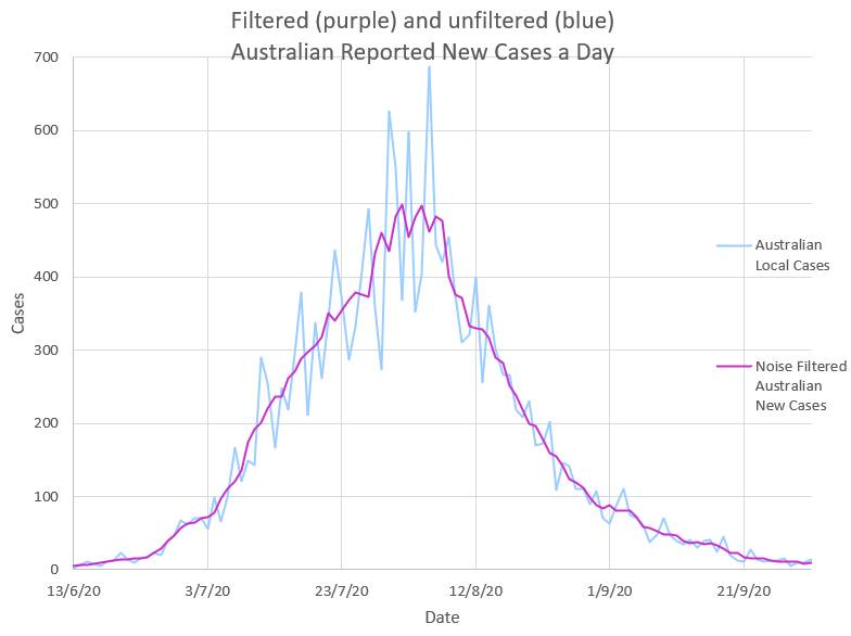
The reported New Cases each day show ‘noise’ and are probably caused by delays in tracing and reporting cases followed by sudden catch up.
|
The ‘noise’ in the daily New Cases can be removed by using a mathematical low pass filter. A mean over 5 days appears to work well. The mean values of N are used in the model. |
|
In practice Rs is volatile and a mean of Rs over 8 days, R8, is more useful as a measure of the reproduction number.
The observed change in Rs, effective R, after Public Health Measures, Non Pharmacologic Interventions, or restrictions are put in place
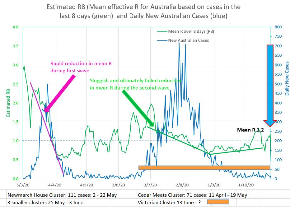
Intuitively it might be expected that Rs would fall rapidly, after a short ‘wash in’ period, to a new stable level after restrictions were put in place . In Australia’s two waves Rs did not behave in that way and it can be noted that in fact Rs appears to fall at a steady almost linear (straight line) rate, or perhaps a back-to-front s shape.
So, when using the Model to project what might happen after an intervention, it may be appropriate to reduce Rs linearly from its current value. Rs (unlike effR) is directly related to the efficacy of the restrictions, EOR. Rs is inversely proportional to the efficacy of the restrictions. EOR = 1 - (Rs/R₀) for Rs between 0 and R₀. The efficacy of restrictions (NPI) drives Rs.
|
The chart shows the rapid but linear like fall in Rs during the first wave, and a slower but linear like fall during the second wave in Australia. |
|
Rs8
The daily Rs (the effective reproduction number or infection ratio of the virus amonst the susceptible) is rather volatile and so a mean of Rs over 8 days, Rs8 or R8, can be used. A value of 1 of Rs or R8 is the threshold above which the infection is spreading epidemically amongst those still susceptible. Rs is not the same concept as effective R (effR, Reff, eR etc) which is simply the new cases divided by the cases which infected them and does not take the population, or the proportion of the population that is susceptible to the infection, into account.
The daily Rs (the effective reproduction number or infection ratio of the virus amonst the susceptible) is rather volatile and so a mean of Rs over 8 days, Rs8 or R8, can be used. A value of 1 of Rs or R8 is the threshold above which the infection is spreading epidemically amongst those still susceptible. Rs is not the same concept as effective R (effR, Reff, eR etc) which is simply the new cases divided by the cases which infected them and does not take the population, or the proportion of the population that is susceptible to the infection, into account.
R₀ , Rs and Rs8 are averages - the actual values of R are probably normally distributed
The actual values of R are probably normally distributed in the population. The number of cases that one person infects is probably dependent on the behaviour and characteristics of that particular person. The average R₀ may be 2.2 but there will probably be individuals who live with large families, have many contacts, frequent crowded place or bars or cafes, take public transport, don't socially distance or wear masks or work multiple jobs, who have much higher personal values for R, (high Rp). And there will be those who are retired, live alone, rarely go out and comply with public health measures who have much lower personal values for R, (low Rp). The average of this distribution would be the apparent effective R, (R₀ or Rs). The virus may spread preferentially through a network of high Rp persons who have behaviours or circumstances in common. High Rp may be a better term than 'super-spreader' because the network effect is probably as important important as the individual's characteristics.
The effect of the distribution of R in the population may explain why the effective Rs appears to be high early in the epidemic (as the virus spreads preferentially in networks of high Rp persons) and why Rs appears to fall slowly and almost linearly over time after restrictions are put in place (perhaps as the distribution and values of Rp change or as lower Rp cases start to become infected by the higher Rp networks).
Types of events or places or occupations may be called 'super spreader' or 'increased spreader'. So events, places, occupations and individuals may range from high R to low R. The number of variables becomes large. In order to consider only one variable, the R of events or places or occupations could be incorporated into the R of the individuals attending those types of events or places or occupations. So, again a person who has a large household or attends bars or large gatherings or travels interstate would have a large personal Rp and an individual retired and living alone may have a low Rp. That is not to say that the events and places or occupations don't contribute to viral spread. They do. But the increase in R is of factored into the personal Rs of the individuals who attend those types of events or places or occupations. The mean of individual Rp would be Rs for that population.
The tendency of an infection to spread rapidly amongst high Rp individuals initially and to include low Rp individuals later may explain why Rs falls more slowly than expected after restrictions are introduced, in a linear or sloping reverse S shaped pattern.
Proportion Needed to Vaccinate
The Proportion Needed to Vaccinate (PNV) is the proportion of the population that needs to be vaccinated to end the epidemic or prevent new epidemic waves or clusters in the absence of public health measures (non-pharmaceutical interventions NPI). It is the proportion (not the number) of the population that must be vaccinated to reduce the the daily case numbers and end the wave or epidemic.
From x = t+8
Nt+10 = Rs * (P – EV - Ct+9)/P * Σ (ax Nx) (Equation A, with vaccination),
x = t
where V (the vaccinated) multiplied by the efficacy of the vaccine E are no longer susceptible. If the vaccine is effective it reduces the number of susceptible individuals much faster than infection does, and the latter (Ct+9) can be ignored.
When x = t+8
Σ (ax Nx)
x = t
is multiplied by 1 or less, the epidemic ends and cannot re-start, since N t+10 would be a steadily decreasing number of new cases.
So, R₀ * (P – EV)/P needs to be 1 (or less), so R₀ * (1 – EV/P) = 1 and
if the vaccine was 100% effective PNV = V/P and would be = 1 - (1/R₀)
So, PNV = (1-1/R₀)/E
But vaccines are not usually 100% effective. So the proportion of the population that needs to be vaccinated, calculated above, needs to be divided by E, the efficacy of the vaccine, which is the proportion of the vaccinated who will not become infected.
PNV would tend to decrease over time because E would appear to increase over time. There would be some 'breakthrough' infections amongst the vaccinated, increasing the non-susceptibility amongst them, from E to a higher value over time.
Saving lives - is it better to impose Restrictions or to Vaccinate?
The answer is surprising.
During the pandemic more lives are saved by introducing public health measures (restrictions, social distancing and mask wearing) than by vaccination. That is because reducing the ability of the virus to spread by lowering the effective reproduction number will immediately start to reduce the number of cases and therefore reduce hospitalizations and deaths. It is also effective because everyone is involved so it works for everyone. Vaccination works on the vaccinated person to remove them from the 'susceptible to the virus' group, but it does not lower the effective reproduction number of the virus.
Once case numbers are low the answer changes. Once case numbers are low the restrictions will not finally end the pandemic (or local part of the pandemic) especially if new cases can 'leak in' from other places and it is difficult to maintain public health measures over very long periods because of the interrelated adverse effects on people's mental and physical health and on the economy. So removing people from the 'susceptible to the virus' group is then very important. Enough of the population needs to be vaccinated as will reduce the effective R of the highest risk group, who have high personal R values, to below 1. Only then can the public health measures (restrictions, social distancing and mask wearing) be eased.
So, in short, introducing restrictions during the pandemic phase will save the most lives and help the most. Not introducing restrictions will cost lives and hospitalizations and hurt the economy. So, introduce adequate restrictions early. But also, restrictions will not be able to be eased until adequate numbers are vaccinated - probably 80% of the population. So get the vaccination program going as vigorously as possible.
Not putting restrictions in place because of a belief that vaccination will do the trick will cost lives and hurt the economy.
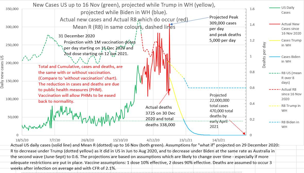
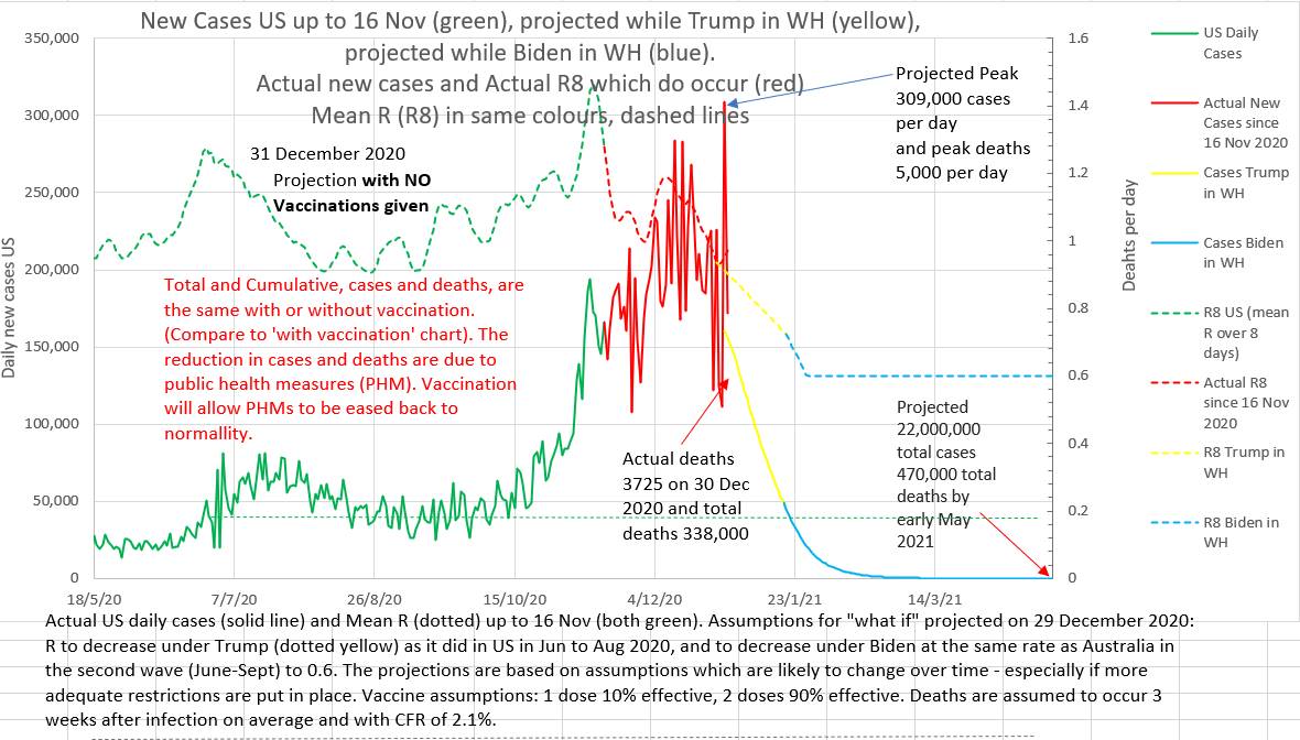
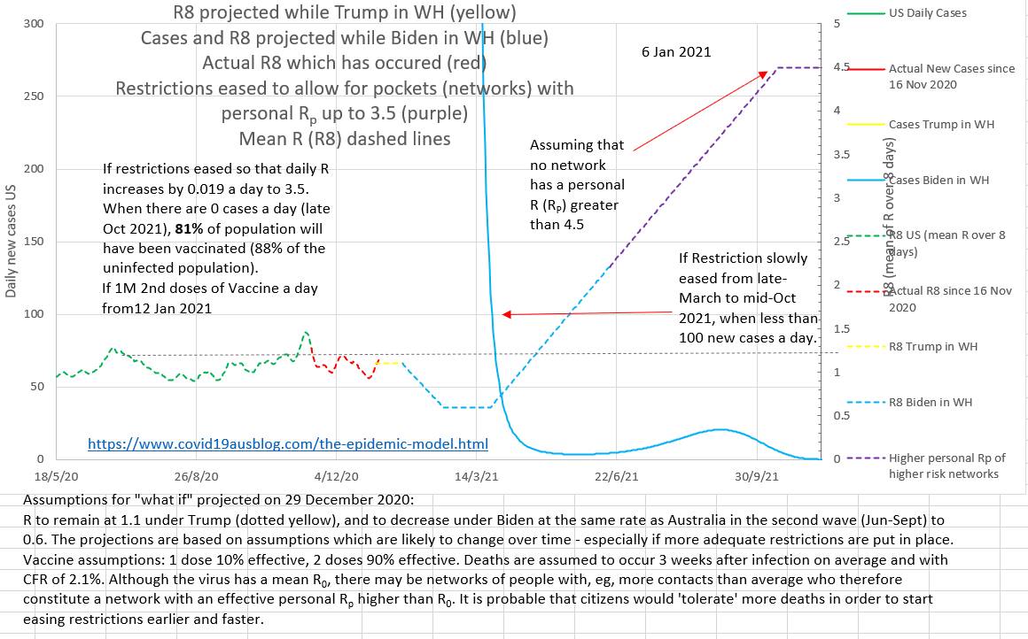
Below are two charts. They are projections made on 29th December 2020. The projection on the left assumes that vaccination will roll out, as planned at that time, at 1 million doses a day. The projection on the right assumes that no vaccinations will be given at all. Note that the total and peak number of cases and deaths are the same with or without vaccination. The projected lowering of cases and deaths is due to the assumed reduction in effective R brought about by public health measures. What these charts do not show is that the epidemic will recur if restrictions are eased before the population is adequately vaccinated.
The answer is surprising.
During the pandemic more lives are saved by introducing public health measures (restrictions, social distancing and mask wearing) than by vaccination. That is because reducing the ability of the virus to spread by lowering the effective reproduction number will immediately start to reduce the number of cases and therefore reduce hospitalizations and deaths. It is also effective because everyone is involved so it works for everyone. Vaccination works on the vaccinated person to remove them from the 'susceptible to the virus' group, but it does not lower the effective reproduction number of the virus.
Once case numbers are low the answer changes. Once case numbers are low the restrictions will not finally end the pandemic (or local part of the pandemic) especially if new cases can 'leak in' from other places and it is difficult to maintain public health measures over very long periods because of the interrelated adverse effects on people's mental and physical health and on the economy. So removing people from the 'susceptible to the virus' group is then very important. Enough of the population needs to be vaccinated as will reduce the effective R of the highest risk group, who have high personal R values, to below 1. Only then can the public health measures (restrictions, social distancing and mask wearing) be eased.
So, in short, introducing restrictions during the pandemic phase will save the most lives and help the most. Not introducing restrictions will cost lives and hospitalizations and hurt the economy. So, introduce adequate restrictions early. But also, restrictions will not be able to be eased until adequate numbers are vaccinated - probably 80% of the population. So get the vaccination program going as vigorously as possible.
Not putting restrictions in place because of a belief that vaccination will do the trick will cost lives and hurt the economy.
Below are two charts. They are projections made on 29th December 2020. The projection on the left assumes that vaccination will roll out, as planned at that time, at 1 million doses a day. The projection on the right assumes that no vaccinations will be given at all. Note that the total and peak number of cases and deaths are the same with or without vaccination. The projected lowering of cases and deaths is due to the assumed reduction in effective R brought about by public health measures. What these charts do not show is that the epidemic will recur if restrictions are eased before the population is adequately vaccinated.
|
|
On the chart below it can be seen that case numbers are already dropping steadily due to restrictions while vaccinations (the blue dotted line right at the bottom right) will only reach 11% of the population by 27th February 2021. The projection was made on the 1st February.
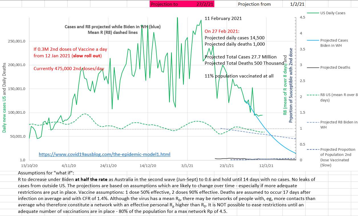
The projection below shows that easing restrictions early or fast may cause a cluster even many months after case numbers have been low.
In Summary
The likely number of new cases on a day can be estimated using Equation A and inputting the number of cases on a day multiplied by the probability of incubation starting on that day, the Rs and the proportion of the population that is still susceptible to infection. Then the calculation can be done again to estimate the next days new cases. The Model is thus discrete and iterative; the equation is used again and again to get the next, then the next, days estimated new cases, each time using cases from earlier days. It is an example of recurrence relation and discrete mathematics (https://mathinsight.org/definition/recurrence_relation) . This is not a single equation Model that estimates the new cases on any particular day in one calculation. This not continuous variable mathematics using simultaneous differential equations.
Equation A:
If the maximum incubation period is 10 (ie i =10),
N t+10 = (0.092 Nt+8 + 0.190 Nt+7 + 0.200 Nt+6 + 0.180 Nt+5 + 0.130 Nt+4 + 0.092 Nt+3 + at+2 Nt+2 + 0.058 Nt+1 + 0.037Nt ) * Rs * (P – C t+9)/P
Where Nt+x are the new cases reported on day t+x. P is the total population, Rs is the number of cases one case infects on average, and C t+9 is the cumulative total cases (all cases) up to day t+9. Initially Rs approximates R₀. The coefficients are the probability that a day is the incubation period for the cases on day t+10, and are obtained from field studies. The probabilities are normalised to add up to 1.
The effective Rs can be estimated from a rearrangement of Equation A, Equation B:
Rs = N t+10 / (0.092 Nt+8 + 0.190 Nt+7 + 0.200 Nt+6 + 0.180 Nt+5 + 0.130 Nt+4 + 0.092 Nt+3 + at+2 Nt+2 + 0.058 Nt+1 + 0.037Nt ) * P/(P – C t+9)
Rs falls in a nearly flat back-to-front 'S' curve which is almost linear after restriction are in place.
The daily reported cases should probably be filtered using a mathematical low pass filter (mean) to reduce noise.