The mathematical viral infection model used in the accompanying blog
Last updated 4th February 2021
Re edited 5 December 2021
It is not possible to use subscripts on this page. The pdf or docx downloads do contain the necessary subscripts.
(c) [email protected]. You have a licence to use, copy, quote or publish this material for any academic or non-commercial purpose with attribution.
Re edited 5 December 2021
It is not possible to use subscripts on this page. The pdf or docx downloads do contain the necessary subscripts.
(c) [email protected]. You have a licence to use, copy, quote or publish this material for any academic or non-commercial purpose with attribution.
Download a docx or pdf of this page here:
The Epidemic Model
The Simple Model
The easy explanation of the Model is in blue. * means multiplied by. The more formal explanation is in black and can be skipped.
At its simplest (and least accurate) the model predicts how many new cases, N, there will be on a day by multiplying the number of cases that are currently secreting the virus (the infecting cases) by a measure of how infectious the virus is (the reproduction number or infection ratio, R) and then multiplying that by the proportion of the population that is still susceptible to the infection. The total population is P. R is the total number of cases infected by one case on average. R in a fully susceptible population is called R0 which for Covid-19 is about 2.2 (and may be up to 3.5).
When the effective R, Re, is estimated from the data and Re over 1 means that the number of cases is increasing exponentially and is an epidemic. An Re under 1 means case numbers are falling. An Re of 1 means that case numbers remain unchanged over time, so either an endemic steady infection or no cases at all.
R0 usually refers to the reproduction number at time zero when the population is completely susceptible. But R0 can be used for other time periods in the equations below because the equations only relate to the remaining susceptible group in the population.
R0 or R varies with the type of infection but also with the behaviour and living conditions in the local population. R will be high in a very mobile, gregarious group where public health measures are poor and low in people who mainly stay at home and comply with public health measures.
New Cases (N) = the infecting cases over the last n days * R0/n * the proportion of the population still susceptible
New Cases (N) = Reported cases over last n days x R0/n x (P – All reported cases)/P
There is often a delay in reporting cases, and then reporting suddenly catches up. This introduces ‘noise’ in the data.
IF it is assumed that those reported as new cases in the last number of days (n) are the only infectious cases that could have infected the new cases on a particular day, then adding up those cases will give the number of infecting cases. Since this model incorporates the decreasing proportion of 'completely susceptible' individuals over time, R remains the same as it did from the start as R0 . R0 is the total number of new infections caused by one infecting case in a wholly susceptible population. As it is assumed that cases are infected by cases that were reported in the previous n days, the daily reproduction number is R0 / n. The potentially susceptible are the whole population P minus every case that has been infected, the cumulative reported cases. Anyone who has had the infection or who currently has the infection is logically not susceptible. They do not need to be declared as recovered. This assumes that very few individuals are infected twice.
IF it is found, for example, that cases are spreading the virus, infectious and infecting, for 6 days, then R0 must be divided by 6 to calculate the spread per day and then counting the days starting at t and the next day as t+1 and the next day as t+2 etc the number of new cases predicted to occur on day t+6 is
N t+6 = (Nt+5 + Nt+4 + Nt+3 + Nt+2 + Nt+1 + Nt ) * R0 /6 * (P – Cumulative Cases t+5)/P
Where Nt+6 means N at sub-scripted time t+6 and R0 means R sub-script 0, the reproduction number in a completely susceptible population or sub-population.
The Use of this Simple Model
|
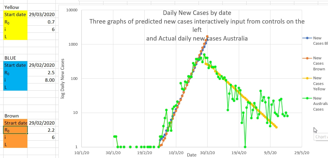
This Simple Model is useful initially when the incubation period and infectious period of the virus is not yet known. Projections using this Model can be 'fitted' against the actual number of cases using various values of R0 and n until the values associated with the 'best fit' are found. Since R0/n must match |
|
the slope of the actual cases (on a log scale) the ratio of R0 to n can be found, and n can be found for a reasonable and plausible value of R0. In addition increasing n increases the number of days over which the 'infecting cases are summed, which alters the shape of the curve slightly. The curve is drawn inputting potential values for R0 and n (here called i) into the coloured boxes to the left of the chart. The curves are 'seeded' with the actual preceding n days cases. The brown curve for R0 of 2.2 and n (or i) of 6 fits slightly better than the blue curve with higher R0 and n. For Covid an R0 of 2.2 and n of 6 days appeared plausible and best fit to the data.
Once restrictions are in place R is affected and R0 can no longer be estimated. But if R0 is known or assumed the Effective R, Re, can be estimated.
Once restrictions are in place R is affected and R0 can no longer be estimated. But if R0 is known or assumed the Effective R, Re, can be estimated.
Improved Model
This formula can be improved for COVID-19 because it has now been shown that the incubation period is 1 to 14 days, and the probability of the incubation taking a particular number of days is known.
Luca Ferretti, Alice Ledda, Chris Wymant et al, ‘The timing of COVID-19 transmission’, September 16, 2020, medRxiv online. At https://doi.org/10.1101/2020.09.04.20188516
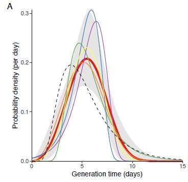
The generation time of Covid-19 (from infected to infected). The incubation period (from infection to symptoms (if any) is shown as a dotted line).
The probability of the incubation being 1 day long is very low, so the probability of having been infected by cases reported the day before are very low. The probability of the incubation being 2 days long is 8.8 percent, so the probability of being infected by the cases reported 2 days before the symptoms is 0.088 or 8.8 percent. And etc for the other days. The probability of having been infected 1 day before or 11 to 15 days before are low, so are not used in the Model. Only the probabilities of infection for days 2 to 10 (numbered t, t+1 etc to t+8) are used in this Model. The probabilities for these 9 days were adjusted to add up to 1 (100%) since you can’t be infected more or less than 100%. These adjusted probabilities are used as coefficients, to multiply by the number of reported cases on that day.
The probability, a, of being infected 1, 2 , 3 etc to 10 days before symptoms (at to at+8) has been found to be 0, 0.092, 0.19, 0.20, 0.18, 0.13, 0.092, 0.058, 0.037 and 0.026% (0%, 9.2, 19, 20, 18,13, 9.2, 5.8, 3.7 and 2.6%) respectively.
So the final equation for Covid-19 (Equation A) is:
N t+10 = (0.092 Nt+8 + 0.190 Nt+7 + 0.200 Nt+6 + 0.180 Nt+5 + 0.130 Nt+4 + 0.092 Nt+3 + at+2 Nt+2 + 0.058 Nt+1 + 0.037Nt ) * R0 * (P – C t+9)/P
Where C t+9 is the cumulative total cases (all cases) up to day t+9,
or,
N t+10 = ADD(ax*Nx for x=t to x=t+8) * R0 * (P – C t+9)/P (Equation A)
Or more formally,
x = t+8
N t+10 = R0 * (P – C t+9)/P * Σ (ax Nx) rearranged (Equation A)
x = t
Where at to at+8 are 0.026, 0.037, 0.058, 0.092, 0.130, 0.180, 0.200, 0.190, and 0.092 respectively.
Since the probabilities (coefficients) are adjusted (normalised) to add up to 1 (100%), it is no longer necessary to divide R0 by n.
Estimating R
If public health measures (restrictions, public health measures) are in place to limit the spread of Covid then the number of cases infected by one case will decrease and the apparent or effective Re replaces R0 in Equation A:
N t+10 = (at+8 Nt+8 + at+8 Nt+8 + at+7 Nt+7 + at+6 Nt+6 + at+5 Nt+5 + at+4 Nt+4 + at+3 Nt+3 + at+2 Nt+2 + at+1 Nt+1 + at Nt ) * Re * (P – C t+9)/P
And an estimated Re can be obtained by rearranging Equation A,
Re = N t+10 / (0.092 Nt+8 + 0.190 Nt+7 + 0.200 Nt+6 + 0.180 Nt+5 + 0.130 Nt+4 + 0.092 Nt+3 + at+2 Nt+2 + 0.058 Nt+1 + 0.037Nt) * P/(P – C t+9)
or more formally,
x = t+8
Re = N t+10 * (P / (P – C t+9)) / Σ (ax Nx) Equation B
x = t
where Nt+10 means N sub-scripted at time t+10, P is the population, Ct+9 is the cumulative total cases on sub-scripted time t+9, ax and Nx mean a and N at sub-script time x.
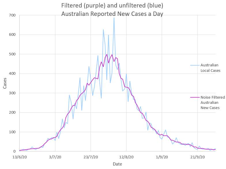
The reported New Cases each day show dips and spikes which are probably ‘noise’ and not real. These are probably caused by delays in tracing and reporting cases followed by sudden catch up. It is important to estimate the number of cases that ‘should have’ been reported on a particular day because new cases on a specific day are multiplied by a specific coefficient, a, in equations A and B.
The probability, a, of being infected 1, 2 , 3 etc to 10 days before symptoms (at to at+8) has been found to be 0, 0.092, 0.19, 0.20, 0.18, 0.13, 0.092, 0.058, 0.037 and 0.026% (0%, 9.2, 19, 20, 18,13, 9.2, 5.8, 3.7 and 2.6%) respectively.
So the final equation for Covid-19 (Equation A) is:
N t+10 = (0.092 Nt+8 + 0.190 Nt+7 + 0.200 Nt+6 + 0.180 Nt+5 + 0.130 Nt+4 + 0.092 Nt+3 + at+2 Nt+2 + 0.058 Nt+1 + 0.037Nt ) * R0 * (P – C t+9)/P
Where C t+9 is the cumulative total cases (all cases) up to day t+9,
or,
N t+10 = ADD(ax*Nx for x=t to x=t+8) * R0 * (P – C t+9)/P (Equation A)
Or more formally,
x = t+8
N t+10 = R0 * (P – C t+9)/P * Σ (ax Nx) rearranged (Equation A)
x = t
Where at to at+8 are 0.026, 0.037, 0.058, 0.092, 0.130, 0.180, 0.200, 0.190, and 0.092 respectively.
Since the probabilities (coefficients) are adjusted (normalised) to add up to 1 (100%), it is no longer necessary to divide R0 by n.
Estimating R
If public health measures (restrictions, public health measures) are in place to limit the spread of Covid then the number of cases infected by one case will decrease and the apparent or effective Re replaces R0 in Equation A:
N t+10 = (at+8 Nt+8 + at+8 Nt+8 + at+7 Nt+7 + at+6 Nt+6 + at+5 Nt+5 + at+4 Nt+4 + at+3 Nt+3 + at+2 Nt+2 + at+1 Nt+1 + at Nt ) * Re * (P – C t+9)/P
And an estimated Re can be obtained by rearranging Equation A,
Re = N t+10 / (0.092 Nt+8 + 0.190 Nt+7 + 0.200 Nt+6 + 0.180 Nt+5 + 0.130 Nt+4 + 0.092 Nt+3 + at+2 Nt+2 + 0.058 Nt+1 + 0.037Nt) * P/(P – C t+9)
or more formally,
x = t+8
Re = N t+10 * (P / (P – C t+9)) / Σ (ax Nx) Equation B
x = t
where Nt+10 means N sub-scripted at time t+10, P is the population, Ct+9 is the cumulative total cases on sub-scripted time t+9, ax and Nx mean a and N at sub-script time x.
The reported New Cases each day show dips and spikes which are probably ‘noise’ and not real. These are probably caused by delays in tracing and reporting cases followed by sudden catch up. It is important to estimate the number of cases that ‘should have’ been reported on a particular day because new cases on a specific day are multiplied by a specific coefficient, a, in equations A and B.
|
The dips and spikes or ‘noise’ in the daily New Cases data, N, can be removed by using a mathematical low pass filter which filters out the high frequency delay and catch up of tracing and reporting. The most effective noise filter is replacing each N with the mean of N over a few days. A mean over 5 days appears to work well. The ‘filtered’ or mean values of N are then used in equation B to obtain the estimated effective Re of the virus. eg Filtered N t+2 = ADD(Nt+4 + Nt+3 + Nt+2 + Nt+1 + Nt) / 5 |
|
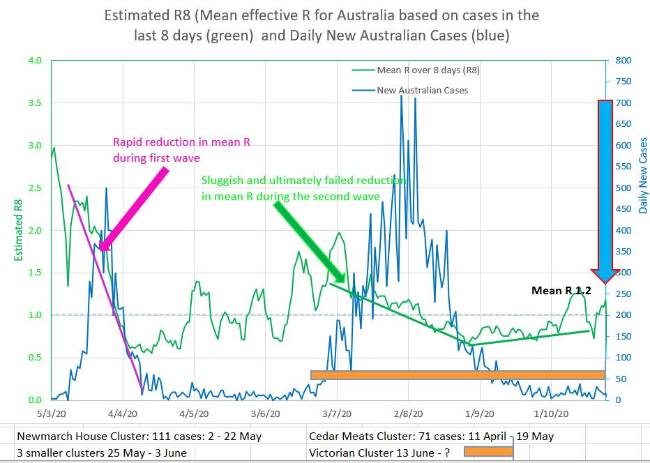
In practice Re is volatile and a mean of Re over 8 days, R8, is more useful as a measure of the reproduction number.
The observed change in Re, effective R, after Public Health Measures, PHM, or restrictions are put in place
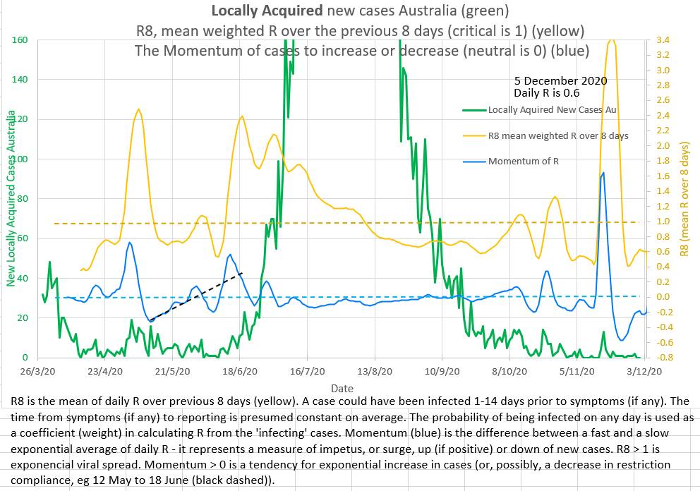
Intuitively it might be expected that Re would fall rapidly, after a short ‘wash in’ period, to a new stable level after restrictions were put in place . In Australia’s two waves Re did not behave in that way and it can be noted that in fact Re appears to fall at a steady almost linear (straight line) rate.
So, when using the Model to project what might happen after an intervention, it may be appropriate to reduce Re linearly from its current value.
|
The chart shows the rapid but linear like fall in Re during the first wave, and a slower but linear like fall during the second wave in Australia. |
|
R8
The daily effective R (Re, the effective reproduction number or infection ratio of the virus) is rather volatile and so a mean of Re over 8 days, R8, can be used. A value of 1 of Re or R8 is the threshold above which the infection is spreading epidemically.
The daily effective R (Re, the effective reproduction number or infection ratio of the virus) is rather volatile and so a mean of Re over 8 days, R8, can be used. A value of 1 of Re or R8 is the threshold above which the infection is spreading epidemically.
R0, Re and R8 are averages - the actual values of R are probably normally distributed
the actual values of R are probably normally distributed in the population. The number of cases that one person infects is probably dependent on the behaviour and characteristics of that particular person. The average R0 may be 2.2 but there will probably be individuals who live with large families, have many contacts, frequent crowded place or bars or cafes, take public transport, don't socially distance or wear masks or work multiple jobs, who have much higher personal values for R, (high Rp). And there will be those who are retired, live alone, rarely go out and comply with public health measures who have much lower personal values for R, (low Rp). The average of this distribution would be the apparent effective R, (R0 or Re). The virus may spread preferentially through a network of high Rp persons who have behaviours or circumstances in common. High Rp may be a better term than 'super-spreader' because the network effect is probably as important important as the individual's characteristics.
The effect of the distribution of R in the population may explain why the effective Re appears to be high or perhaps over-estimated, early in the epidemic (as the virus spreads preferentially in networks of high Rp persons) and why Re appears to fall slowly and almost linearly over time after restrictions are put in place (perhaps as the distribution and values of Rp change or as lower Rp cases start to become infected by the higher Rp networks) rather than quickly after a short wash-in period as might be expected.
|
Momentum
Momentum (in blue on this chart) attempts to measure the upward or downward momentum or impetus on the number of new cases a day. More positive values suggest an upward impetus driving cases numbers up, and more negative numbers suggest a downward impetus driving cases down. It is similar to a stock price indicator called MACD invented by Gerald Appel in the 1970s. |
|
A slow moving exponential moving average of the number of cases a day is subtracted from a fast moving exponential moving average of the number of cases a day to obtain the Momentum.
The exponential moving average is calculated by adding a fraction of a day's new cases to the complementary fraction of the previous average. For the fast exponential moving average 30% of the number of new cases that day are added to 70% of yesterday's fast exponential moving average. Or FEMA = (0.3 * new cases) + (1 - 0.3) * previous FEMA. For the slow moving exponential moving average 15% of the number of new cases that day are added to 85% of yesterday's slow exponential moving average. Or SEMA = (0.15 * new cases) + (1 - 0.15) * previous SEMA. Momentum is obtained by subtracting SEMA from FEMA. Momentum = FEMA - SEMA.
Note that the new cases on a day contribute the most (30%) to the FEMA on the day they occur and then they contribute less the next day (contributing 70% of 30% or 21%) and less again to the FEMA on the next day (70% of 70% of 30% or 14%) and so on. If case numbers remain static the Momentum returns to zero.
Acceleration
Acceleration is taken to be the Momentum less the Momentum the day before. A = Mt+1 - Mt
Acceleration is taken to be the Momentum less the Momentum the day before. A = Mt+1 - Mt
Number Needed to Vaccinate
The Number Needed to Vaccinate (NNV) is the proportion of the population that needs to be vaccinated to end the epidemic or prevent new epidemic waves or clusters in the absence of public health measures (PHM or non-pharmaceutical interventions NPI). It is the proportion (not the number) of the population that must be vaccinated to reduce the R below 1 among those who are susceptible to the virus. R even lower would be safer. The problem is deciding which R to use.
Often the whole population is considered susceptible unless vaccinated, probably for abundant caution.
Then from x = t+8
Nt+10 = R0 * (P – V)/P * Σ (ax Nx) rearranged (Equation A),
x = t
where V (the vaccinated) are no longer susceptible.
When x = t+8
Σ (ax Nx)
x = t
is multiplied by 1 or less, the epidemic ends and cannot re-start, since N t+10 would be a steadily decreasing number of new cases.
So, R0 * (P – V)/P needs to be 1 (or less), so R0 * (1 – V/P) = 1
and V/P is the proportion needed to vaccinate and is 1 - (1/R0)
But, R0 is the average or mean R of the population. Some members of the population will have behaviours that increase their personal R, Rp. And these people are probably more likely to network in some way (they like bars, use public transport, have multiple jobs, come from big families, etc). They may have an Rp of 3.5 or 4.5 or more. So the greatest personal R of a significant subset of the population, gRp should probably be used in the calculation.
So the NNV is probably 1 - (1/gRp) which is a greater proportion of the population than 1 - (1/R0).
But, most of those who have been infected already (C, the cumulative total cases to date) will probably not be susceptible (at least not in the short term),
so, R0 * (P – V - C)/P needs to be 1 (or less)
and the number needed to vaccinate NNV = V/P
is 1 - (1/gRp) - (C/P)
The question is then which R to use?
The average R among the susceptible in the population, R0, may be 2.2 for example, but there will be individuals and networks of individuals with higher personal R values, Rp. The R to use is likely the highest Rp that is present in a significant subset of the population. The Rp to use may well be 3.5 or even 4.5. If the virus mutates and it results in higher R values (more infectious) then even higher Rp values may need to be used to calculate the NNV (the proportion of the population that need to be vaccinated).
If Rp is R0 = 2.2 the NNV = 54% of the population
If the likely network high Rp is 3.5 the NNV = 71% of the population
If the likely network high Rp is 4.5 the NNV = 78% of the population
If the likely network high Rp is 4.5 and 28 of 330 million of the population has been infected the NNV = 1 - (1/Rp) - (C/P)
which is 70% of the population. 70% of the whole population, although the vaccine would not generally be given initially to those who had already been infected.
Finally, allowance should be mad for the fact that the vaccine may not be 100% effective. So the proportion of the population that needs to be vaccinated (NNV) calculated above needs to be divided by E, the efficacy of the vaccine, which is the proportion of the vaccinated who do not infect others.
For example, if 90% of those vaccinated appear not to infect others, then in this context E is 0.9 and the number (in fact the proportion) needed to vaccinate, NNV, is the NNV calculated above divided by 0.9.
So, finally, if NNV is 0.8 (80%) from the above calculations, and the efficacy, E, of the vaccine is 0.9, the the actual NNV (proportion) is 0.8/0.9 which is about 0.9 (90%).
Saving lives - is it better to impose Restrictions or to Vaccinate?
The answer is surprising.
During the pandemic more lives are saved by introducing public health measures (restrictions, social distancing and mask wearing) than by vaccination. That is because reducing the ability of the virus to spread by lowering the effective reproduction number will immediately start to reduce the number of cases and therefore reduce hospitalizations and deaths. It is also effective because everyone is involved so it works for everyone. Vaccination works on the vaccinated person to remove them from the 'susceptible to the virus' group, but it does not lower the effective reproduction number of the virus.
Once case numbers are low the answer changes. Once case numbers are low the restrictions will not finally end the pandemic (or local part of the pandemic) especially if new cases can 'leak in' from other places and it is difficult to maintain public health measures over very long periods because of the interrelated adverse effects on people's mental and physical health and on the economy. So removing people from the 'susceptible to the virus' group is then very important. Enough of the population needs to be vaccinated as will reduce the effective R of the highest risk group, who have high personal R values, to below 1. Only then can the public health measures (restrictions, social distancing and mask wearing) be eased.
So, in short, introducing restrictions during the pandemic phase will save the most lives and help the most. Not introducing restrictions will cost lives and hospitalizations and hurt the economy. So, introduce adequate restrictions early. But also, restrictions will not be able to be eased until adequate numbers are vaccinated - probably 80% of the population. So get the vaccination program going as vigorously as possible.
Not putting restrictions in place because of a belief that vaccination will do the trick will cost lives and hurt the economy.
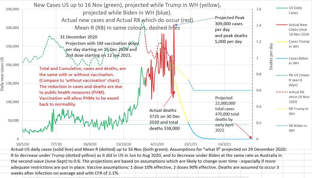
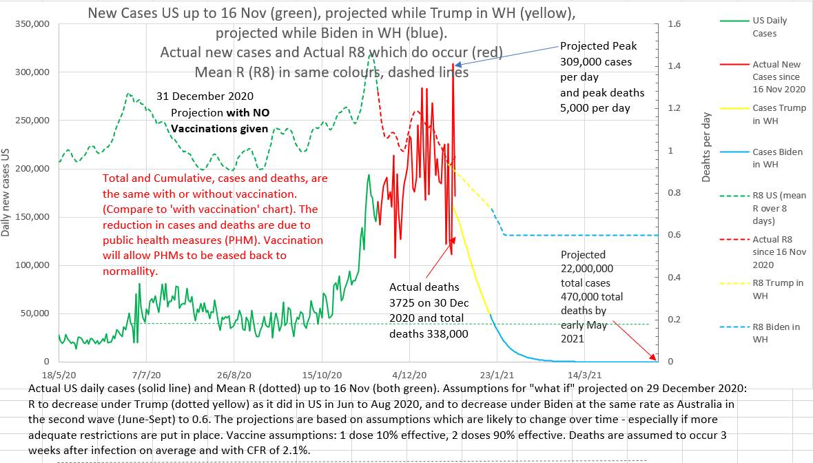
Below are two charts. They are projections made on 29th December 2020. The projection on the left assumes that vaccination will roll out, as planned at that time, at 1 million doses a day. The projection on the right assumes that no vaccinations will be given at all. Note that the total and peak number of cases and deaths are the same with or without vaccination. The projected lowering of cases and deaths is due to the assumed reduction in effective R brought about by public health measures. What these charts do not show is that the epidemic will recur if restrictions are eased before the population is adequately vaccinated.
The answer is surprising.
During the pandemic more lives are saved by introducing public health measures (restrictions, social distancing and mask wearing) than by vaccination. That is because reducing the ability of the virus to spread by lowering the effective reproduction number will immediately start to reduce the number of cases and therefore reduce hospitalizations and deaths. It is also effective because everyone is involved so it works for everyone. Vaccination works on the vaccinated person to remove them from the 'susceptible to the virus' group, but it does not lower the effective reproduction number of the virus.
Once case numbers are low the answer changes. Once case numbers are low the restrictions will not finally end the pandemic (or local part of the pandemic) especially if new cases can 'leak in' from other places and it is difficult to maintain public health measures over very long periods because of the interrelated adverse effects on people's mental and physical health and on the economy. So removing people from the 'susceptible to the virus' group is then very important. Enough of the population needs to be vaccinated as will reduce the effective R of the highest risk group, who have high personal R values, to below 1. Only then can the public health measures (restrictions, social distancing and mask wearing) be eased.
So, in short, introducing restrictions during the pandemic phase will save the most lives and help the most. Not introducing restrictions will cost lives and hospitalizations and hurt the economy. So, introduce adequate restrictions early. But also, restrictions will not be able to be eased until adequate numbers are vaccinated - probably 80% of the population. So get the vaccination program going as vigorously as possible.
Not putting restrictions in place because of a belief that vaccination will do the trick will cost lives and hurt the economy.
Below are two charts. They are projections made on 29th December 2020. The projection on the left assumes that vaccination will roll out, as planned at that time, at 1 million doses a day. The projection on the right assumes that no vaccinations will be given at all. Note that the total and peak number of cases and deaths are the same with or without vaccination. The projected lowering of cases and deaths is due to the assumed reduction in effective R brought about by public health measures. What these charts do not show is that the epidemic will recur if restrictions are eased before the population is adequately vaccinated.
|
|
On the chart below it can be seen that case numbers are already dropping steadily due to restrictions while vaccinations (the blue dotted line right at the bottom right) will only reach 11% of the population by 27th February 2021. The projection was made on the 1st February.
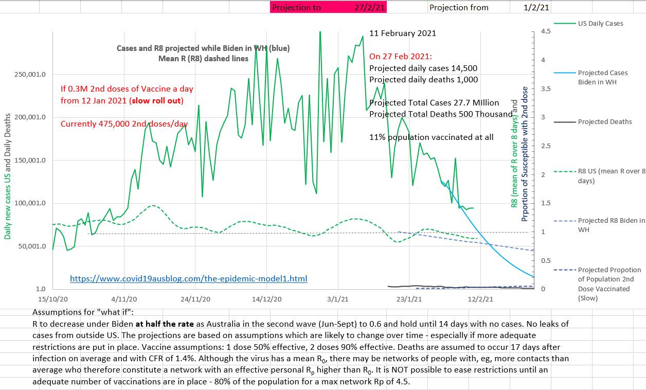
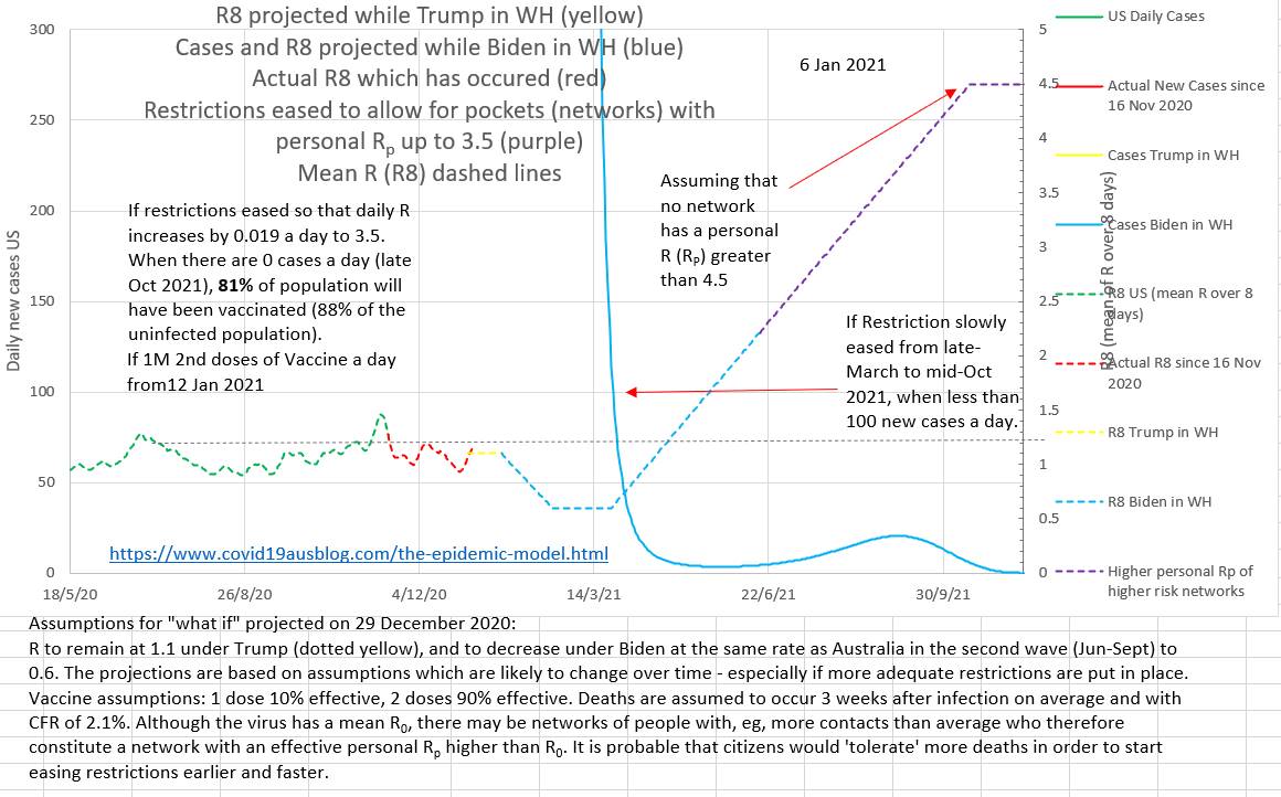
The projection below shows that easing restrictions early or fast may cause a cluster even many months after case numbers have been low.
In Summary
The likely number of new cases on a day can be estimated using Equation A and inputting the number of cases from nine earlier days. Then the calculation can be done again to estimate the next days new cases. The Model is thus iterative; the equation is used again and again to get the next, then the next, days estimated new cases, each time using cases from earlier days. It is an example of recurrence relation and discrete mathematics (https://mathinsight.org/definition/recurrence_relation) . This is not a single equation Model that estimates the new cases on any day in one calculation. This not continuous variable mathematics.
Equation A:
N t+10 = (0.092 Nt+8 + 0.190 Nt+7 + 0.200 Nt+6 + 0.180 Nt+5 + 0.130 Nt+4 + 0.092 Nt+3 + at+2 Nt+2 + 0.058 Nt+1 + 0.037Nt ) * R0 * (P – C t+9)/P
Where Nt are the new cases reported on day t. P is the total population, R0 is the number of cases one case infects on average when all the population is susceptible, and C t+9 is the cumulative total cases (all cases) up to day t+9,
The effective Re can be estimated from Equation B:
Re = N t+10 / (0.092 Nt+8 + 0.190 Nt+7 + 0.200 Nt+6 + 0.180 Nt+5 + 0.130 Nt+4 + 0.092 Nt+3 + at+2 Nt+2 + 0.058 Nt+1 + 0.037Nt ) * P/(P – C t+9)
Re falls in a nearly linear fashion after restriction are in place.
The daily reported cases should probably be filtered using a mathematical low pass filter to reduce the noise of delay and catch up of tracing and reporting. Replacing N with a mean value of the data around N (say a mean of 5 values centered on N) appears viable. The mean is apparently the best noise reducing filter.
